Gradient Descent
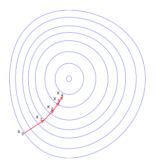
Gradient descent is an iterative optimization algorithm that minimizes a function (such as a neural network's loss function) by repeatedly moving the parameters in the direction opposite to the gradient of the function at the current point. Because the gradient points toward the steepest ascent, subtracting it from the parameters moves the model toward a local (or global) minimum. Variants like Stochastic Gradient Descent (SGD) and Adam are the workhorses of modern deep learning training.
Key Formula
theta[t+1] = theta[t] - learning_rate * gradient_of_loss_at_theta[t]
LaTeX: \theta_{t+1} = \theta_t - \alpha \nabla_\theta L(\theta_t)
| Symbol | Meaning | Unit |
|---|---|---|
| \theta_t | Model parameters (weights and biases) at step t | dimensionless |
| \alpha | Learning rate (step size) | dimensionless |
| \nabla_\theta L | Gradient of the loss with respect to parameters | dimensionless |
Worked Example
Problem
Minimize the function L(w) = w² + 4w + 4 using gradient descent. Start at w₀ = 3 with learning rate α = 0.1. Perform 3 update steps.
Solution
Step 0 — Gradient: dL/dw = 2w + 4 Step 1 (t=0): w = 3 Gradient = 2(3) + 4 = 10 w₁ = 3 − 0.1 × 10 = 3 − 1 = 2.0 Step 2 (t=1): w = 2 Gradient = 2(2) + 4 = 8 w₂ = 2 − 0.1 × 8 = 2 − 0.8 = 1.2 Step 3 (t=2): w = 1.2 Gradient = 2(1.2) + 4 = 6.4 w₃ = 1.2 − 0.1 × 6.4 = 1.2 − 0.64 = 0.56 Note: The true minimum is at w = −2 (where dL/dw = 0), so the algorithm converges toward −2.
Answer
After 3 steps: w ≈ 0.56, converging toward minimum at w = −2
Gradient Descent Variants Compared
| Variant | Batch Size | Update Frequency | Pros / Cons |
|---|---|---|---|
| Batch GD | Full dataset | Once per epoch | Stable but slow on large data |
| Stochastic GD (SGD) | 1 sample | Once per sample | Fast but noisy updates |
| Mini-batch GD | 32–512 samples | Once per mini-batch | Best trade-off, most used |
| Adam | Mini-batch | Adaptive per parameter | Fast convergence, widely used |
| RMSProp | Mini-batch | Adaptive learning rate | Good for RNNs |
Interactive Tools
Wikimedia Commons, CC BY-SA
Related Terms
Backpropagation
Backpropagation (backward propagation of errors) is the algorithm used to train neural networks by efficiently computing the gradient of the loss function with respect to every weight in the network. It applies the chain rule of calculus in a reverse pass through the network — from the output layer back to the input layer — so that each weight can be updated in the direction that reduces the loss. Without backpropagation, training deep neural networks with millions of parameters would be computationally infeasible.
Neural Network
A neural network is a computational model loosely inspired by the structure of biological brains, consisting of layers of interconnected nodes (neurons) that process and transform data. Each neuron computes a weighted sum of its inputs, applies a non-linear activation function, and passes the result to the next layer. Neural networks are the foundation of modern AI and are capable of learning highly complex patterns in images, text, audio, and tabular data.
Overfitting
Overfitting occurs when a machine learning model learns the training data too well — including its noise and random fluctuations — to the point where it performs poorly on new, unseen data. An overfitted model has high training accuracy but low validation/test accuracy, indicating it has memorized patterns specific to the training set rather than generalizing. Overfitting is more likely with complex models, small datasets, or insufficient regularization.
"Gradient" derives from Latin "gradus" (step). The gradient descent algorithm in the context of optimization was described by Augustin-Louis Cauchy in 1847 as the "method of steepest descent." Its application to neural network training was established in the 1980s.