PID Controller
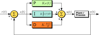
A PID (Proportional-Integral-Derivative) controller is a feedback control mechanism that calculates a control output based on three terms: the proportional term (current error), the integral term (accumulated past error), and the derivative term (rate of change of error). Together these three components allow the controller to eliminate steady-state error, respond rapidly to disturbances, and suppress oscillations. PID controllers are the most widely used feedback controllers in industrial automation, motor drives, temperature regulation, and robotic systems due to their effectiveness and relative simplicity of tuning.
Key Formula
u(t) = Kp·e(t) + Ki·∫e(τ)dτ + Kd·de(t)/dt
LaTeX: u(t) = K_p\,e(t) + K_i\int_0^t e(\tau)\,d\tau + K_d\,\frac{de(t)}{dt}
| Symbol | Meaning | Unit |
|---|---|---|
| u(t) | Control output signal | Varies (V, %, N, etc.) |
| e(t) | Error = setpoint − measured output | Varies |
| K_p | Proportional gain | Dimensionless |
| K_i | Integral gain | 1/s |
| K_d | Derivative gain | s |
Worked Example
Problem
A temperature control system uses a PID controller with Kp = 2, Ki = 0.5 /s, Kd = 0.1 s. At t = 5 s, the error is e(5) = 3°C, the integral of error over [0,5] is 10 °C·s, and de/dt = −1 °C/s. Calculate the controller output u(5).
Solution
Step 1: Calculate the proportional term. P = Kp · e(t) = 2 × 3 = 6 Step 2: Calculate the integral term. I = Ki · ∫e dt = 0.5 × 10 = 5 Step 3: Calculate the derivative term. D = Kd · de/dt = 0.1 × (−1) = −0.1 Step 4: Sum all three terms. u(5) = P + I + D = 6 + 5 + (−0.1) = 10.9
Answer
u(5) = 10.9 (in controller output units, e.g., 10.9% of heater power or 10.9 V)
Effect of PID Gain Tuning on System Response
| Parameter Increase | Rise Time | Overshoot | Settling Time | Steady-State Error |
|---|---|---|---|---|
| K_p ↑ | Decreases | Increases | Small change | Decreases |
| K_i ↑ | Decreases | Increases | Increases | Eliminated |
| K_d ↑ | Small effect | Decreases | Decreases | No effect |
| All three balanced | Fast | Minimal | Short | Zero |
Interactive Tools
Wikimedia Commons, CC BY-SA
Related Terms
Feedback Control
Feedback control is a control strategy in which the output of a system is measured and compared to a desired reference (setpoint), and the difference (error) is used to adjust the system input to reduce that error. Negative feedback — where the output is subtracted from the reference — is the basis of stable automatic control systems in engineering, biology, and economics. Feedback control enables systems to self-correct against disturbances and parameter variations, forming the foundation of servo systems, thermostats, autopilots, and industrial process control.
Transfer Function (control)
A transfer function is the ratio of the Laplace transform of the output to the Laplace transform of the input of a linear time-invariant (LTI) system, assuming zero initial conditions. It fully characterises a system's dynamic behaviour in the frequency domain, including its poles, zeros, gain, and stability margins. Transfer functions are the central tool in classical control theory for designing feedback controllers, analysing stability using root locus and Bode plots, and predicting transient and steady-state responses.
Laplace Transform
The Laplace Transform converts a time-domain function into the complex frequency domain (s-domain), enabling differential equations to be solved as algebraic equations. It generalises the Fourier Transform by including a real exponential damping term, making it applicable to a broader class of signals including those that grow with time. It is the primary mathematical tool in control systems engineering, circuit analysis, and linear system theory for analysing stability, transient response, and frequency behaviour.
PID is an acronym for Proportional-Integral-Derivative. The proportional control concept was introduced by Nicolas Minorsky in 1922 while studying automatic ship steering. The full three-term controller was formalised by Taylor Instrument Companies and Foxboro Company in the 1930s for industrial process control. Ziegler and Nichols published their famous empirical PID tuning rules in 1942, which remain widely used today.